Machine Learning and Simulated Annealing
There’s no doubt you’ve heard of machine learning. It seems like every new tech company claims that they are going be the ones to solve an impossible problem by just letting their computers figure it out. It’s a miracle! Machine learning is a big buzzword right now. It sounds simple enough to say that you are going to “use machine learning”, but how exactly does a machine learn? In short, the answer is that, much like humans, machines learn through trial and error. We must give the machine some actions, parameters, and tests so it can rate its success. The machine remembers successful choices and tries to do things in a similar way in the future, inching slowly toward a solution. Various machine learning models exist, but as an introduction, we will discuss a simple model called simulated annealing.

The Tour Guide
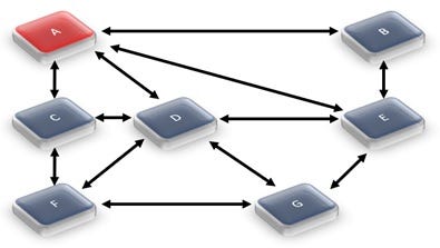
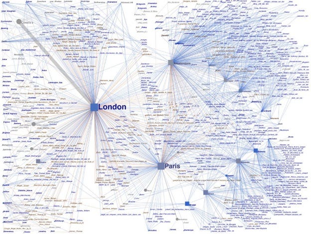
To understand simulated annealing, put yourself in the shoes of a tour guide carrying tourists through the map in figure 1. You pick up a group of people at point A who have hired you to drive them to destinations B through G. The passengers want to visit each location once and need to return to point A at the end of the trip. They are also on a tight sightseeing schedule and want you to minimize their travel distance to reduce travel time. The only way between points is by taking the connecting roads, represented as lines in the diagram. How do you optimize your trips? This might seem like an easy problem for so few points, but complexity quickly skyrockets as you add more destinations and roads. Figure 2 is a perfect example — an exhaustive trial-and-error approach (driving every possible path) might take years of travel. Suddenly the number of choices is so great that it’s impossible to solve on paper — or even with a computer algorithm that compares every possible solution. This is where simulated annealing comes into play.

Simulated annealing is a technique that is used to find the best solution for either a global minimum or maximum, without having to check every single possible solution that exists. This is super helpful when addressing massive optimization problems like the one previously stated. Let’s take a look at where this idea came from before we get into the explanation of how it works.
Origins of Simulated Annealing
Simulated annealing actually has its origins in metallurgy. In metallurgy, annealing refers to the process of heating metal to a high temperature and then slowly cooling it in a controlled environment. The high heat gives the atoms in the metal the freedom to move around wildly. If the metal were to be cooled quickly, the atoms would suddenly come to rest wherever they were when the metal was hot, resulting in a random arrangement and a poor quality result. But when the metal is cooled slowly, the atoms have time to gradually find the best possible orientation, and align themselves into a nice crystal lattice. This is preferable to quick cooling; it makes the metal more ductile, reduces defects, and makes it significantly stronger (2). In general, annealing gradually reduces energy and movement to allow a substance’s components to settle into their most stable, simplest order.

With this in mind, consider our tour guide example and imagine randomly connecting locations on your map into a potential “best route”. Your route is built from a series of aimless, hastily-made connections and is quite likely not a good route at all. This parallels “quick cooling” — you have locked in some random choices in the same way that atoms might be stopped in their random positions in a metal — this results in a bad solution. However, if you slowly “cool” your route, and continually decide to trade out longer roads for shortcuts, you may be able to progressively reduce travel time and find the shortest possible path.
The Algorithm
The mindful route choice is essentially how a simulated annealing algorithm works. For our tour guide example, you would first randomly map out a limited number of paths that reach every destination and quantify each of them with a total travel time. For these unique paths, you would then branch out and try similar variations, and again check the travel time. If your travel time goes down, you’re taking a step in the right direction and update your path! But what do you do if your travel time increases? It could very well be the case that variations on that longer-travel-time path would be better than variations on the existing path. To account for this, you initially decide to accept longer-travel-time routes very frequently. As you try out more and more paths, you decide to be less and less forgiving of paths that increase travel time. This is like the slow cooling in metal annealing — as you lower the figurative “temperature,” you get pickier, and allow progressively less chaos in your solution. Eventually, after a set number of attempts, your “temperature” reaches the predefined minimum and you stop drawing new paths. The path with the lowest travel time at the end of your sampling is your optimized route. Problem solved!
Translating these tasks into a program makes sense — this kind of repetitive sampling and comparing work is perfect for a computer. Using a computer allows you to sample more and compare faster, which increases the likelihood of finding a better route. Simulated annealing isn’t just useful for travelling problems, either! It can be applied to problems in almost any field, including the type of biotechnology work we do at Macromoltek. Simulated annealing is often used to make predictions about how a protein will fold (within some margin of error). There are many variables to be considered, but with enough sampling and with the right parameter adjustments, we can develop a framework from this technique that will optimize the deep learning algorithms. Together this is what is commonly referred to as machine learning.
Links and Citations:
1. Figure 2. Network diagram of agents connecting the British, Belgian, Dutch, and French auction markets from 1801–1820 using 230,000 records from the Getty Provenance Index databases. © J. Paul Getty Trust and Maximilian Schich. http://www.getty.edu/research/tools/
2. Verhoeven, J.D. Fundamentals of Physical Metallurgy, Wiley, New York, 1975, p. 326

Looking for more information about Macromoltek, Inc? Visit our website at www.Macromoltek.com
Interested in molecular simulations, biological art, or learning more about molecules? Subscribe to our Twitter and Instagram!
